Introduction to rasterly

library(rasterly)
library(data.table)
library(lubridate)
library(grid)
library(plotly)

rasterly makes it easy to rapidly generate raster images for large datasets. Although the package is inspired by the Datashader library available for Python, rasterly does not attempt to reproduce all the features of Datashader. Rather, rasterly offers comparable performance to Datashader when generating rasters from source data. rasterly attempts to provide a flexible, convenient interface which should feel familiar to users of ggplot2 and its aesthetics-based approach to customizing plots and figures.

A raster may be described as a matrix of cells or pixels arranged in grid-like fashion, in which each pixel represents a value in the source data. When combined with the package and Plotly.js, rasterly enables analysts to generate interactive figures with very large datasets which are responsive enough to embed into Dash for R applications.

The rasterly function creates a rasterly object, to which aggregation layers may be added. This function is the first step in the process of generating raster image data using the package. The rasterly function is not intended to be used in isolation, since aggregation layers are required for full functionality.

Data set

The dataset used in this vignette describes Uber trips taken in New York City from April 1st to September 30th of 2014.

# Load data
ridesRaw_1 <- "https://raw.githubusercontent.com/plotly/datasets/master/uber-rides-data1.csv" %>%
  data.table::fread(stringsAsFactors = FALSE)
ridesRaw_2 <- "https://raw.githubusercontent.com/plotly/datasets/master/uber-rides-data2.csv" %>% 
  data.table::fread(stringsAsFactors = FALSE)
ridesRaw_3 <- "https://raw.githubusercontent.com/plotly/datasets/master/uber-rides-data3.csv"  %>% 
  data.table::fread(stringsAsFactors = FALSE)
ridesDf <- list(ridesRaw_1, ridesRaw_2, ridesRaw_3) %>% 
  data.table::rbindlist()

# Extract hour of trip taken
time <- lubridate::ymd_hms(ridesDf$`Date/Time`)
ridesDf <-  ridesDf[, 'Date/Time':=NULL][, list(Lat, 
                                                Lon,
                                                hour = lubridate::hour(time), 
                                                month = lubridate::month(time),
                                                day = lubridate::day(time))]

This dataset has 4,533,327 observations, and includes the variables “latitude”, “longitude”, “hour”, “month” and “day”.

Basic

If we were to use graphics::plot(), it would take several minutes to render the image. What if we “rasterized” the image instead?

start_time <- Sys.time()
p <- ridesDf %>% 
  rasterly(mapping = aes(x = Lat, y = Lon)) %>% 
  rasterly_points()
p
end_time <- Sys.time()
end_time - start_time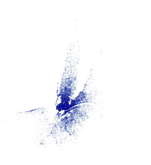

A raster image, in essence, is a large sparse matrix and each element is a hexadecimal color (A character vector with elements of 7 or 9 characters, “#” followed by the red, blue, green and optionally alpha values). Since the range (x, y) of this display can be acquired, we can also map the image into a data.frame with mapping coordinates x, y and color. For example:

image <- as.raster(matrix((1:4)/4, nrow = 2))
image

##      [,1]      [,2]     
## [1,] "#404040" "#BFBFBF"
## [2,] "#808080" "#FFFFFF"

# mapping this image onto a 1 <= x <= 2 and 2 <= y <= 5 plane
rasterly::image2data(image, x_range = c(1, 2), y_range = c(2, 5))

##    x y   color
## 1: 1 5 #404040
## 2: 1 2 #808080
## 3: 2 5 #BFBFBF
## 4: 2 2 #FFFFFF

In this way, we can transform a large dataset (million or billion) into a raster image (say 400 \(\times\) 400), then, mapping this image to a data.frame but dropping blank ones. So the size can decrease from 160000 to rough 30k or 40k (It really depends on data). In other word, we can always reduce a huge size to a reasonable size and the darkness of color is judged by the “Reduction Function” (see section ‘API’ for more info)

imageData <- rasterly::image2data(p)
# basic graphics 
# It is slow but still much faster than drawing the huge data directly)
plot(x = imageData$x, y = imageData$y, col = imageData$color)

`rasterly` Structure

Subsetting

rasterly() generates a parent layer containing initial settings to generate the raster, which include plot_height, plot_width among others; child layers such as rasterly_points() can be piped in as well. Note that “p” above is a list of environments. The elements in “p” can be easily extracted or replaced by [ and [<-.

p["background"]
# $rasterly_env
# [1] "white"

# $rasterlyPoints1
# [1] "white"
########### Replace the background in child layer `rasterly_points()`
p["background", level = 2] <- "black"
p["background"]
# $rasterly_env
# [1] "white"

# $rasterlyPoints1
# [1] "black"
########## Colors in both `rasterly()` and `rasterly_points()` are replaced
## fire is a vector of colors (as character strings) with length 256
## see `rasterly::fire`
p["color", level = 1:2] <- fire_map
p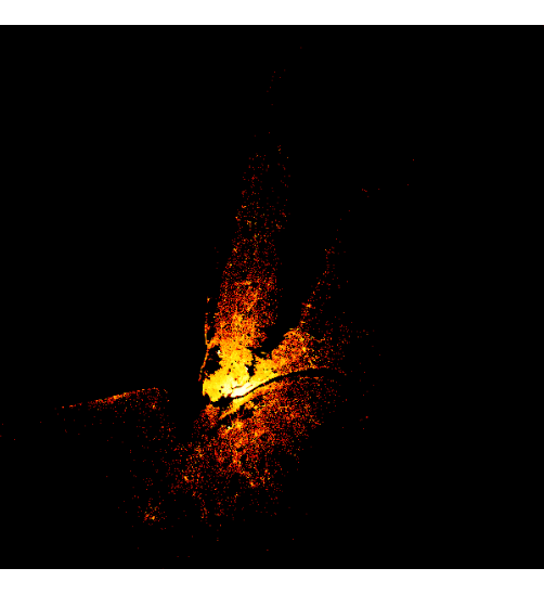

level helps to define which layer to replace; the default is 1 (the parent layer generated by rasterly()).
Available states which can be extracted or replaced are listed here:
1. Aggregation: data, mapping, plot_width, plot_height, range, x_range, y_range, xlim, ylim, aesthetics, reduction_func, glyph, max_size, group_by_data_table, drop_data, variable_check
2. Display: background, color, alpha, span, show_raster, layout

Build rasterly by `rasterly_build()`

To retrieve display info, use rasterly_build():

build <- rasterly_build(p)
str(build)

It contains:

agg: aggregation matrices, a list of numerical matrices
image: a raster matrix (has the same dimension with aggregation matrices)
lims: a list of x limits and y limits for each layer
x_range: the range of x over all layers
y_range: the range of y over all layers
plot_height: plot height, number of rows in aggregation matrix
plot_width: plot width, number of columns in aggregation matrix
variable_names: names of variables
background: background color
colors: color used to map in each pixel or used for categorical variable. It is distinguished by whether “color” is set in aes() or not

Display

rasterly does not provide any functionality to display the raster image data it generates, but instead relies on other packages.

`plotly` graphics

add_rasterly_heatmap(): Layers are added to Plotly objects via add_trace(...); rasterly provides the add_rasterly_heatmap() function which also leverages add_heatmap() to generate single channel heatmap overlays for Plotly figures. Multi-channel heatmaps are not currently supported; this feature will be available in an upcoming release.
```
plotly::plot_ly(ridesDf, x = ~Lat, y = ~Lon) %>%
  add_rasterly_heatmap() %>% 
  layout(
    title = "Uber drives",
    xaxis = list(
      title = "Lat"
    ),
    yaxis = list(
      title = "Lon"
    )
  )
```

plotRasterly(): plotRasterly has very similar API with rasterly but return a plotly object.

# if as_image is FALSE, the image will be transformed to a data.frame
plotRasterly(ridesDf, 
             mapping = aes(x = Lat, y = Lon),
             as_image = TRUE)

`ggplot` graphics

ggRasterly takes the arguments from rasterly and returns a ggplot object. In this case, image will be transformed to a data.frame automatically.

ggRasterly(data = ridesDf, 
           mapping = aes(x = Lat, y = Lon, color = hour),
           color = hourColors_map) + 
  labs(title = "New York Uber",
       subtitle = "Apr to Sept, 2014",
       caption = "Data from https://raw.githubusercontent.com/plotly/datasets/master")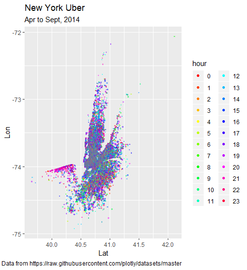

API

rasterly application programming interface

r <- rasterly(data = ridesDf, 
                mapping = aes(x = Lat, y = Lon))

Mapping system

Set color

Different colors represent different hours:

r %>% 
  rasterly_points(
    mapping = aes(color = hour),
    color = hourColors_map,
    background = "black"
  ) -> g
# `plot(g)` involves axes and legend as well
plot(g, xlab = "latitude", ylab = "longitude", 
     main = "Visualization of NYC Uber Rides in 2014",
     legend_main = "hour",
     legend_label = 0:23)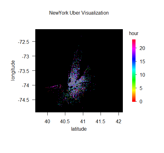

The colors attribute in “image” within build_g is generated via weighted arithmetic means (default) computed from the aggregation matrices. We can choose the “cover” layout to display multiple aggregation matrices:

r %>% 
  rasterly_points(
    mapping = aes(color = hour),
    color = hourColors_map,
    background = "black",
    layout = "cover"
  ) -> g
plot(g, xlab = "latitude", ylab = "longitude", 
     main = "Visualization of NYC Uber Rides in 2014",
     legend = FALSE)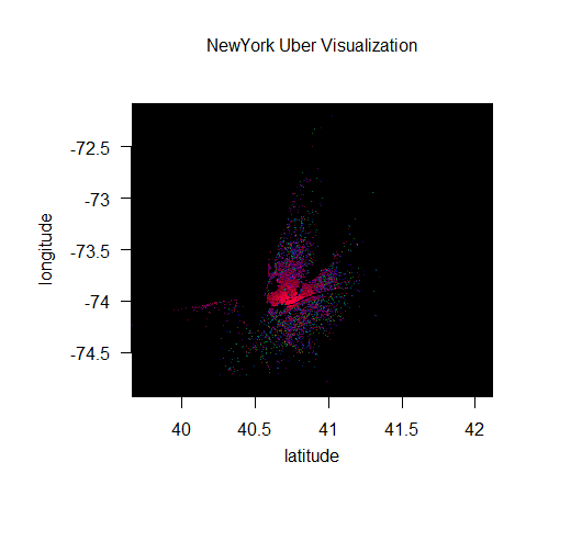

The resulting raster will be overlaid onto the plotting surface.

Set on

reduction_func is implemented on which variable

r %>% 
  rasterly_points(
    # take the "mean" reduction function 
    # more details are in section 'Reduction function'
    reduction_func = "mean", 
    mapping = aes(on = -Lat)
  )

Set size

To control the number of pixels allocated to an observation, we can set the size aesthetic; when specified, the max_size argument provides the upper bound of the number of pixels a single observation is allocated:

r %>% 
  rasterly_points(
    mapping = aes(size = month),
    max_size = 4
  )

Currently, only x, y, color, on and size can be set using aes().

Reduction function

A reduction operator function is used when aggregating data points within each bin. One option is to reduce using the mean of the points.

mean reduction function:

r %>% 
  rasterly_points(
    reduction_func = "mean", # process the data points using the mean reduction function
    background = "black",    # change background to "black" from right to left (from dark to light)
    color = fire_map # provide a custom color_map
  )

The mean reduction function averages the y column (default setting) for every observation. It’s also possible to average over other features using the on aesthetic; consult the list of available reduction functions below for additional details.

any reduction function:

# zoom in
r %>% 
  rasterly_points(
    reduction_func = "any",
    color = c("white", "black")
  ) %>% 
  plot(xlim = c(40.3, 41.3))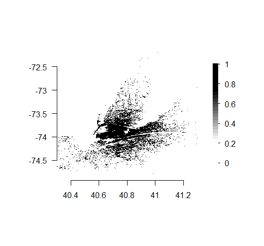

Currently supported reduction functions:

sum: If on is not provided within aes(), the default is to take the sum within each bin. When on is specified, the function reduces by taking the sum of all elements within the variable named in on.
any: When on is provided within aes(), the any reduction function specifies whether any elements in on should be mapped to each bin.
mean: If on is not provided in mapping aes(), on would be set as variable “y” by default. When on is given, the mean reduction function takes the mean of all elements within the variable specified by on.

The following functions require that on is first provided via aes():

m2: The m2 function computes the sum of square differences from the mean of all elements in the variable specified by on.
var: The var function computes the variance over all elements in the vector specified by on.
sd: The sd function computes the standard deviation over all elements in the vector specified by on.
first: The first function returns the first element in the vector specified by on.
last: The last function returns the last element in the vector specified by on.
min: The min function returns the minimum value in the vector specified by on.
max: The min function returns the maximum value in the vector specified by on.

Zehao Xu

2020-06-04

Data set

Basic

`rasterly` Structure

Subsetting

Build rasterly by `rasterly_build()`

Display

`plotly` graphics

`ggplot` graphics

API

Mapping system

Reduction function

Contents

Introduction to rasterly

Zehao Xu

2020-06-04

Data set

Basic

rasterly Structure

Subsetting

Build rasterly by rasterly_build()

Display

plotly graphics

ggplot graphics

API

Mapping system

Reduction function

Contents

`rasterly` Structure

Build rasterly by `rasterly_build()`

`plotly` graphics

`ggplot` graphics